RAG Architecture in Production

What is RAG?

Retrieval-Augmented Generation combines a language model with a retrieval system. The model doesn't generate from memory alone. it retrieves relevant context from an external knowledge base, then uses that context to generate responses.

In practice, RAG is a pipeline: chunk documents into manageable pieces, embed those chunks into a vector space, retrieve the most similar chunks to a user query, and feed them to the model alongside the question. The result is responses grounded in your actual data rather than model's training corpus.

RAG Architecture at a Glance

• Combines retrieval systems with LLMs to ground responses
• Uses vector search to find relevant context
• Improves accuracy, reduces hallucinations
• Requires careful handling of latency and evaluation

Deep dive: RAG Core Components

When to Use RAG vs Fine-Tuning

This is the first architectural decision, and most teams get it wrong. The common misconception is that fine-tuning teaches the model new knowledge or controls its style. In practice, fine-tuning serves a different purpose entirely.

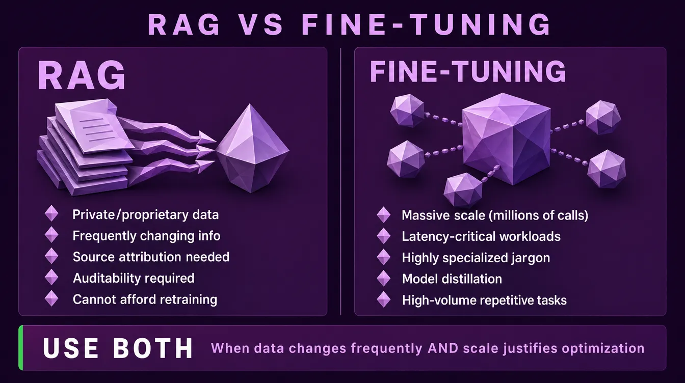
Use RAG when:

• Your data is private, proprietary, or specific to your organization
• Information changes frequently (policies, products, documentation)
• You need source attribution and verifiable responses
• You require traceability and auditability
• You cannot afford to retrain a model every time something changes

Use fine-tuning when:

• You operate at massive scale (millions of API calls) and need to reduce per-query token costs
• Latency is critical and you need to eliminate lengthy system prompts
• Your domain has highly specialized jargon, codes, or terminology that the base model consistently misreads
• You want to distill a smaller model to behave like a larger one for a specific task
• You have a high-volume, repetitive task requiring deterministic output

The pattern: fine-tuning optimizes for efficiency and consistency at scale, not for knowledge injection or output style.

A common myth: Fine-tuning is often pitched as the way to control tone, voice, or output format. In practice, a well-crafted system prompt handles those requirements without the cost and maintenance overhead of training. Fine-tuning for style is almost always the wrong tool.

Use both when: You have frequently changing data (RAG) and high enough scale to justify a fine-tuned generation model for cost efficiency. This combination is rare but valid for high-throughput production systems.

Deep dive: The RAG Decision: When to Choose RAG Over Fine-Tuning

When RAG Isn't the Right Tool

RAG is not a universal foundation for AI systems. Treating it as one is a common architectural mistake.

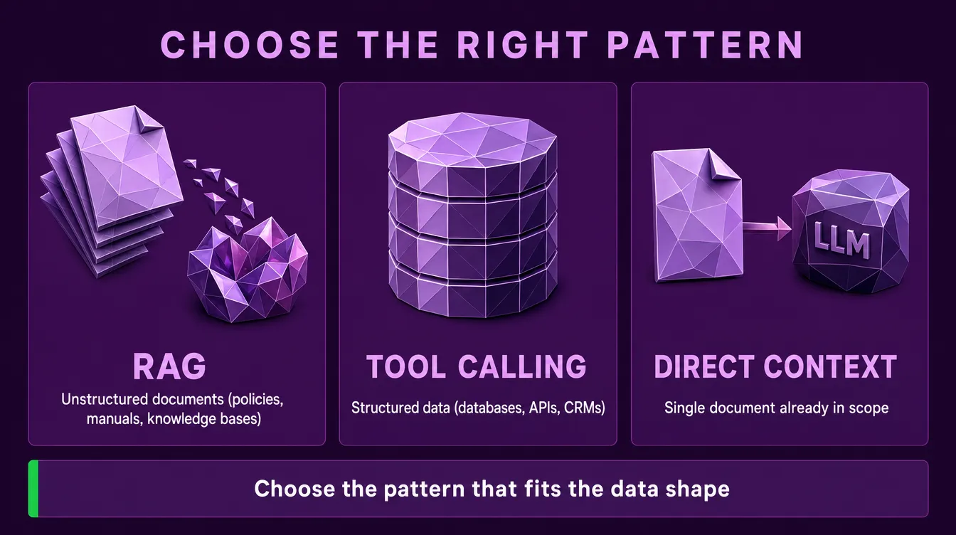
RAG is purpose-built for unstructured document retrieval: policies, manuals, knowledge bases, articles, support documentation. When the question is "what does our documentation say about X," RAG is the right pattern.

RAG is the wrong tool when:

• Data is structured (databases, APIs, CRMs). Tool calling and direct query translation produce more accurate, deterministic results than embedding rows and searching for them.
• Documents are already in hand. If the user has uploaded a single contract or report, just pass it to the LLM directly. Chunking and embedding a single document adds complexity without benefit.
• Questions require computation, aggregation, or filtering ("how many tickets did we close last quarter"). These are SQL queries, not retrieval problems.

The right architecture often combines patterns: RAG for unstructured corpora, tool calling for structured data, direct context loading for individual documents in scope. Choosing the right pattern per data type is more important than picking a single approach for the whole system.

Core Architecture Overview

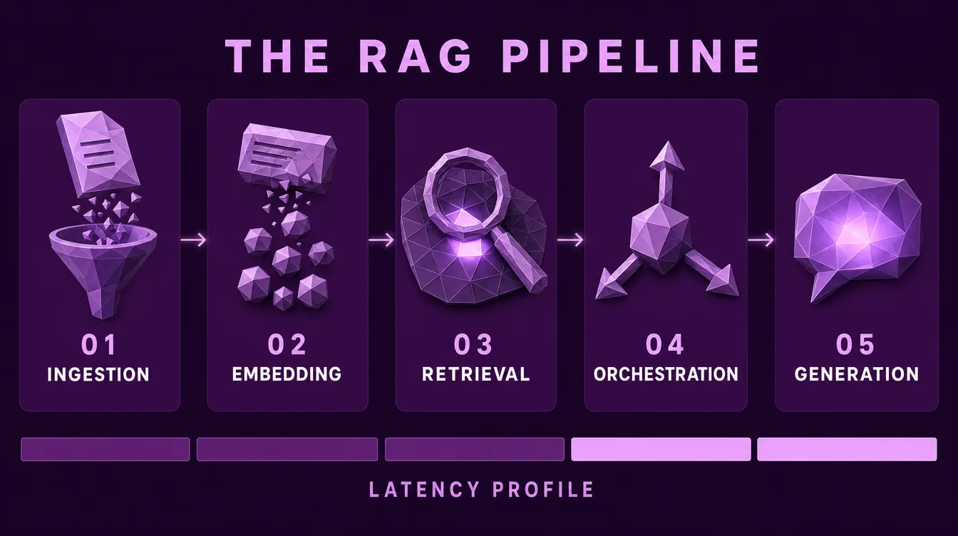
A production RAG system has five core stages:

1. Ingestion . extracting and cleaning data from source systems
2. Embedding . converting chunks into vectors
3. Retrieval . finding relevant chunks for a query
4. Orchestration . routing, reranking, and context assembly
5. Generation . producing the final response

Each stage has different scaling characteristics, failure modes, and latency profiles. Treat them as independent components that can be swapped, not a monolithic pipeline.

Deep dive: RAG Architectures - From Basic to Big Brain Mode

Ingestion Pipeline

The retrieval system is only as good as what's indexed. Ingestion is where most production RAG systems fail.

Chunking strategy matters more than embedding model choice. The Goldilocks zone for most use cases is 200-500 tokens per chunk, large enough to preserve meaningful context, small enough to keep embeddings focused. Q and A over documentation typically performs best at 256-512 tokens. Legal, compliance, and code documentation may benefit from larger chunks (512-1024 tokens) to preserve full clauses or function definitions. Structured data often should not be chunked at all. Direct query translation works better.

Data quality enforcement is critical. Garbage in, garbage out applies absolutely to RAG. If low-quality content reaches the index, retrieval cannot clean it up. Implement validation at ingestion: detect duplicates, flag low-quality content, normalize encoding issues, strip headers and footers, and extract metadata for filtering.

Update cadence depends on use case. Some systems need near-realtime indexing; others can batch daily or weekly. Do not over-engineer indexing speed if updates are infrequent. Match the pipeline to the actual rate of change.

Deep dive: Chunking: The Foundation of Retrieval Quality

Embeddings

The embedding model converts text into vectors. These vectors define the search space for retrieval.

Model selection: BGE, OpenAI's text-embedding-3 family, Cohere's embed-v3, and Google's text-embedding-004 all perform well across most use cases. The recall difference between top performers is small in production. Consistency, latency, and operational fit usually matter more than marginal benchmark differences.

Dimension count: Higher dimensions can improve recall but increase storage cost and retrieval latency. The right dimension count depends on corpus size and query patterns; benchmark on your own data rather than defaulting to whatever the API offers.

Normalization: Most modern embedding models produce normalized vectors. Confirm this in the model documentation. If normalization is required and not applied, cosine similarity calculations break.

Dense vs sparse: Dense embeddings capture semantic similarity. Sparse methods (BM25, SPLADE) handle exact keyword matching, proper nouns, and rare terms. Hybrid approaches combining both typically outperform either alone in production, at the cost of additional operational complexity.

Deep dive: Embeddings & Vector Databases

Retrieval Layer

Retrieval is often the bottleneck. The most common failure mode is over-fetching, returning too many chunks, which dilutes relevance and inflates generation latency.

Top-k tuning: Do not default to k=10. The right k depends on chunk size and question complexity. For most systems, k=3-5 final chunks sent to the LLM is sufficient. More chunks introduce more noise into the context window.

Threshold-based filtering: Instead of (or alongside) top-k, filter by similarity score threshold. This handles edge cases where relevant documents simply do not exist in the index. Better to return nothing than return irrelevant matches.

Reranking: Two-stage retrieval is the production standard. Retrieve a broader set of candidates with a fast bi-encoder (vector search), then rerank with a cross-encoder model that scores query-document pairs precisely. This combines the scalability of vector search with the accuracy of cross-encoding.

Query understanding: User queries are often short, ambiguous, or use different vocabulary than the indexed documents. Query rewriting, expansion, decomposition, and HyDE (hypothetical document embeddings) can substantially improve retrieval quality before the search even runs.

Deep dive: Query Processing: Getting the Question Right

Orchestration

Orchestration is the control layer between retrieval and generation. It decides what context is sent to the model and how.

Context assembly: Assemble retrieved chunks into a structured prompt. Include document citations for traceability. Chunk ordering matters. Chronological order often produces better answers than relevance order for multi-document questions.

Handling retrieval failures: When no relevant chunks are found, the system should clearly indicate that the answer is not available in the knowledge base rather than hallucinate from the model's training data. For high-stakes use cases (legal, medical, financial), saying "I don't know" is the correct behavior. Falling back to general model knowledge should be an explicit, marked decision, not a default.

Multi-turn conversation: Chat history changes the retrieval target. Approaches include rewriting the current query using prior turns, retrieving across the full conversation, or using specialized memory architectures. Choose based on actual conversation patterns observed in production, not theoretical elegance.

Guardrails: Input filtering (prompt injection prevention), output filtering (sensitive content blocking), and query classification (routing to appropriate handlers) are not optional in production deployments.

Generation

The generation model produces the final response. Model selection here involves different trade-offs than embedding or reranking.

Model size: Larger models follow instructions better and use context more reliably, but cost more and run slower. For many RAG use cases, a mid-sized model with strong context handling outperforms a larger model without RAG. Strong retrieved context compensates for raw model capability.

Context window: Newer models offer 128K+ token context windows. This enables longer contexts but introduces challenges. Attention complexity grows quadratically, and effective context utilization degrades well before the theoretical limit. Test actual performance, not advertised capacity.

Temperature and sampling: For factual RAG responses, use low temperature (0.0-0.3). Higher temperatures introduce variability that often manifests as hallucination, even with strong retrieval. Reserve higher temperatures for creative or exploratory use cases.

Structured output: When you need JSON or a specific format, use models with native structured output support or apply schema validation. Do not rely on prompting alone for output structure.

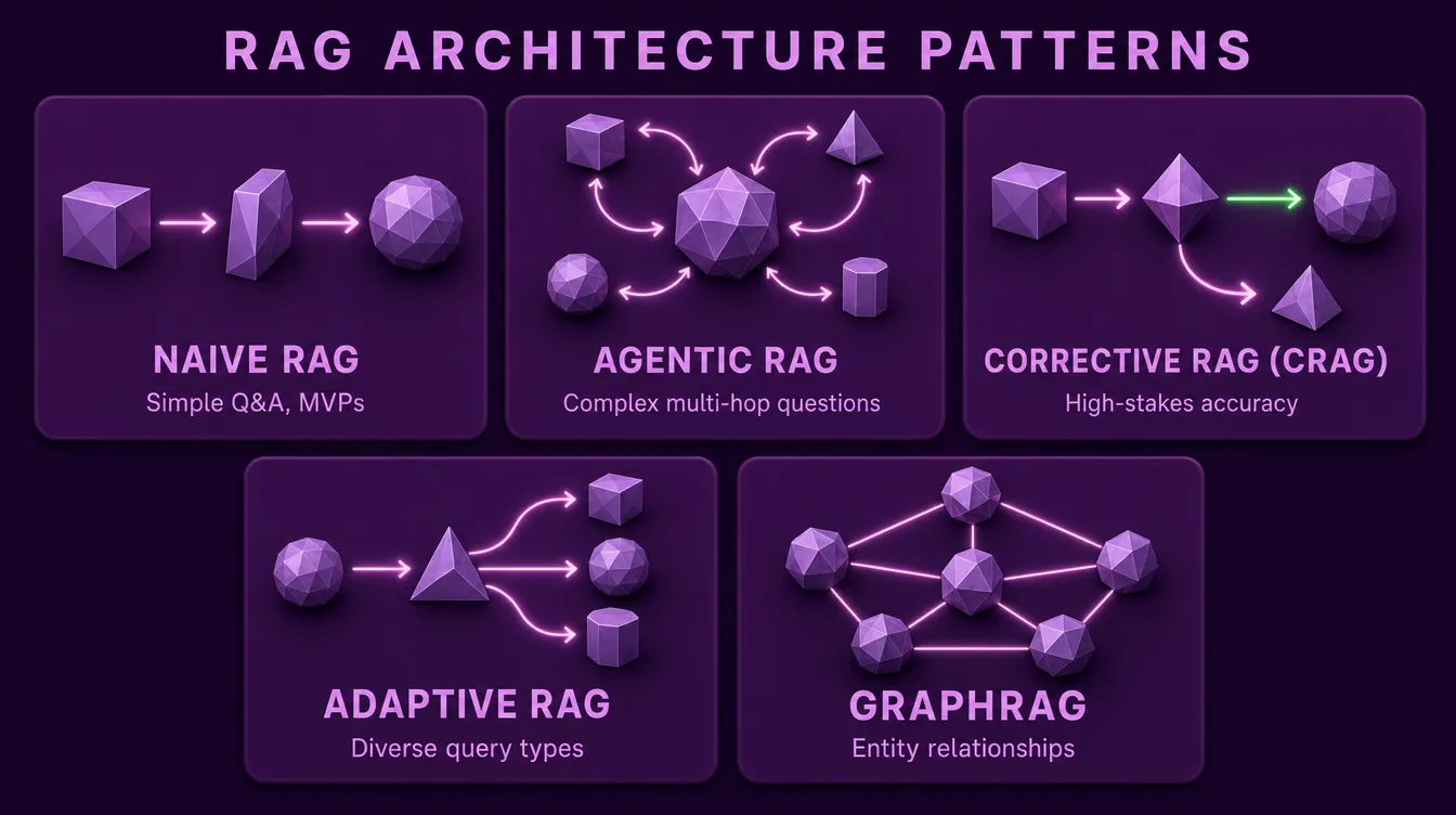
RAG Architecture Patterns

Not all RAG systems are built the same way. Different query patterns and accuracy requirements call for different architectures. Understanding the patterns helps you match complexity to the actual problem.

Naive RAG

The starting point. A single retrieval step feeds the LLM, which generates the response. No reranking, no query rewriting, no self-correction.

When to use: MVP and prototype phases, simple factual Q and A over a clean knowledge base, predictable query patterns, low-latency requirements.

Limitations: Cannot handle complex multi-step questions, no recovery when retrieval fails, single strategy applied to all query types regardless of fit.

Naive RAG handles a surprisingly large share of real-world queries. Do not add complexity until production data shows it needed.

Agentic RAG

An LLM-controlled retrieval loop. Instead of a fixed pipeline, the LLM decides what to retrieve, when to retrieve it, whether to retrieve at all, and when it has enough information to answer. The model becomes an agent reasoning over the retrieval process itself.

When to use: Open-ended research assistance, complex multi-hop questions, exploratory analysis, scenarios where queries require different retrieval strategies that cannot be predetermined.

Trade-offs: Higher latency from multiple LLM calls, harder to debug, more expensive per query. The flexibility costs predictability.

Corrective RAG (CRAG)

Adds an evaluation step after retrieval. A relevance evaluator scores the retrieved documents. If they pass, generation proceeds normally. If they fail, the system triggers a fallback (web search, alternate retrieval strategy, or refusal to answer).

When to use: Legal, medical, financial, and compliance contexts where wrong answers are unacceptable. Situations where saying "I don't know" is preferable to a confident but wrong response.

Trade-offs: Extra LLM call adds latency and cost. The accuracy gain is significant for high-stakes use cases but unnecessary for casual ones.

Adaptive RAG

A query classifier routes incoming requests to the most appropriate retrieval strategy. Simple factual queries go through a fast naive path. Complex comparisons trigger query decomposition. Critical questions route through CRAG. Greetings skip retrieval entirely.

When to use: Production systems serving diverse query types, particularly when query volume is high enough that optimizing the average case yields meaningful cost and latency improvements.

Trade-offs: More moving parts, more pipelines to maintain, classifier accuracy becomes a critical dependency.

GraphRAG

Replaces (or augments) vector similarity with knowledge graph traversal. Documents are processed into entities and relationships; retrieval follows graph edges rather than vector distance.

When to use: Questions where entity relationships matter: organizational structures, regulatory dependencies, citation networks, supply chains, anything where the answer requires understanding how things connect rather than what they say.

Trade-offs: Significantly higher ingestion complexity (extracting entities and relationships from documents), graph database operational overhead, harder to update incrementally.

Choosing an Architecture

Situation	Architecture	Key Benefit
Prototype or MVP	Naive RAG	Simplicity, fast to ship
Mostly simple queries	Naive RAG	Low latency, low cost
Accuracy is critical	CRAG	Self-correction, safe fallbacks
Complex, exploratory queries	Agentic RAG	Dynamic reasoning
Diverse query types at scale	Adaptive RAG	Optimized per query
Entity relationships matter	GraphRAG	Connection-aware retrieval

The right pattern is the simplest one that solves your actual problem. Add architectural complexity only when production failures justify it.

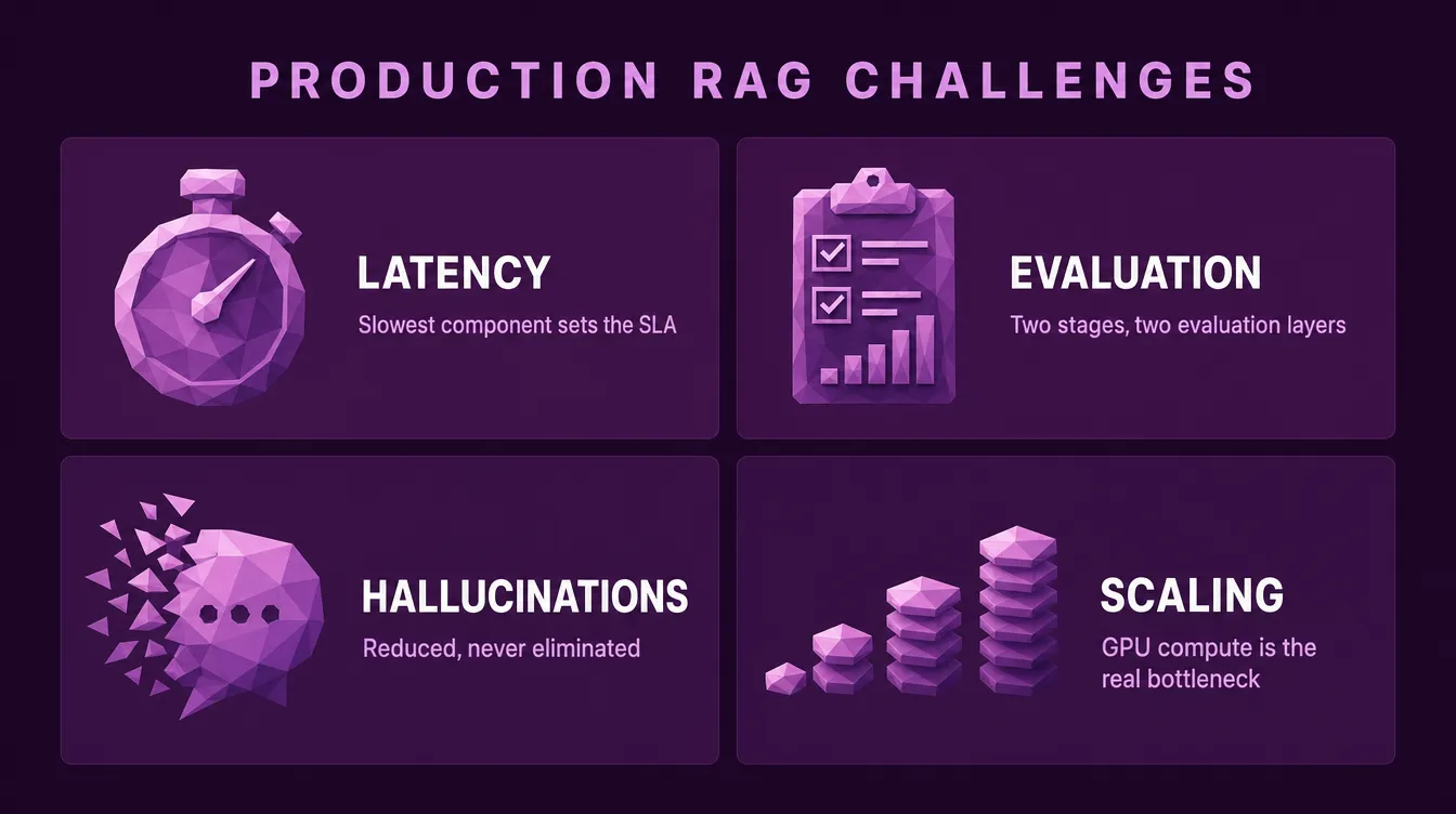
Production Challenges

Four challenges trip up most production RAG deployments:

Latency

End-to-end latency is the sum of retrieval (milliseconds), reranking (milliseconds to a second), and generation (typically seconds). The slowest component sets the SLA. For interactive use cases, target under 2 seconds total. Profile each component independently. Retrieval is often faster than expected, generation is often slower.

Evaluation

RAG evaluation differs from standard LLM evaluation. The system has two stages that fail independently, so both need separate quality measurement.

Retrieval metrics:

• Recall: did we find all relevant documents?
• Precision: of what we found, how much was actually relevant?
• MRR (Mean Reciprocal Rank): how high in the ranking is the best document?
• NDCG (Normalized Discounted Cumulative Gain): overall ranking quality across multiple relevant documents

Deep dive: Advanced retrieval

Generation metrics:

• Faithfulness: is the answer grounded in retrieved documents, or did the model hallucinate?
• Relevance: does the answer actually address the question?
• Completeness: did the answer cover everything needed?
• Conciseness: is the answer focused, or padded with unnecessary content?

LLM-as-judge approaches work for automated evaluation but require careful prompt design to avoid bias. Combine with periodic human evaluation for ground truth.

Deep dive: How to Know If Your RAG System Is Actually Good (And Keep It That Way)

Hallucinations

RAG reduces hallucinations but does not eliminate them. The model may ignore retrieved context, conflate details across chunks, or generate from its own training data. Mitigations: enforce citations in the output, verify generated claims against retrieved content, and test faithfulness as a primary metric, not just "does the answer look right."

Scaling

Vector search scales sub-linearly with index size but linearly with query rate. For high-volume systems, the embedding and generation models become the bottleneck (GPU compute), not the vector store. Plan for horizontal scaling of inference endpoints separately from the vector database. Caching at every layer (embeddings, retrieval results, generations) typically yields larger gains than infrastructure tuning.

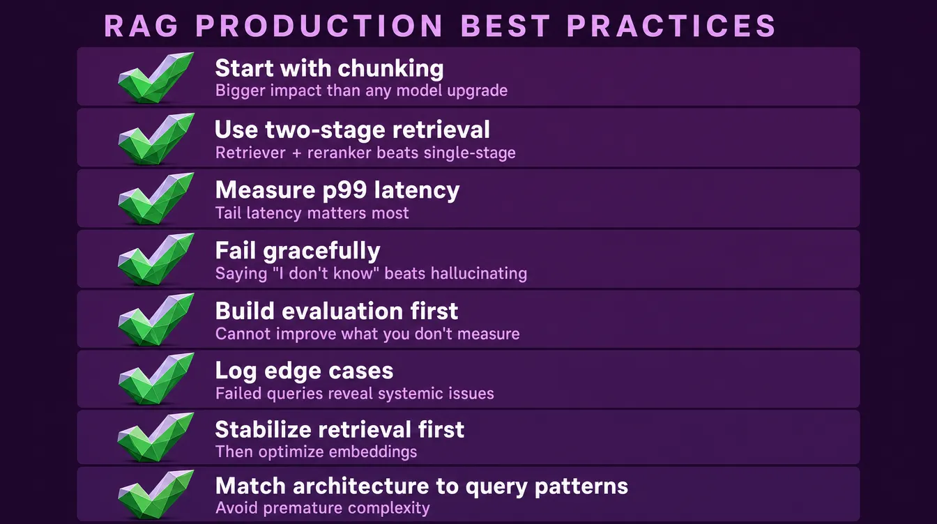
Best Practices

What works in production:

• Start with chunking. The right chunking strategy improves retrieval more than any embedding model upgrade.
• Use two-stage retrieval. Retriever plus reranker outperforms single-stage retrieval for any precision-critical use case.
• Measure end-to-end latency at p99, not average. Tail latency matters most for interactive systems.
• Fail gracefully. When retrieval fails, the system should say so, not hallucinate.
• Build evaluation before optimization. You cannot improve what you do not measure.
• Log and review edge cases. Failed queries reveal systemic issues faster than aggregate metrics.
• Do not optimize the embedding model before the retrieval pipeline is stable. Retrieval issues compound downstream and obscure the impact of model changes.
• Match architecture to query patterns. Most systems do not need GraphRAG or full agentic loops. Add complexity when failure data demands it.

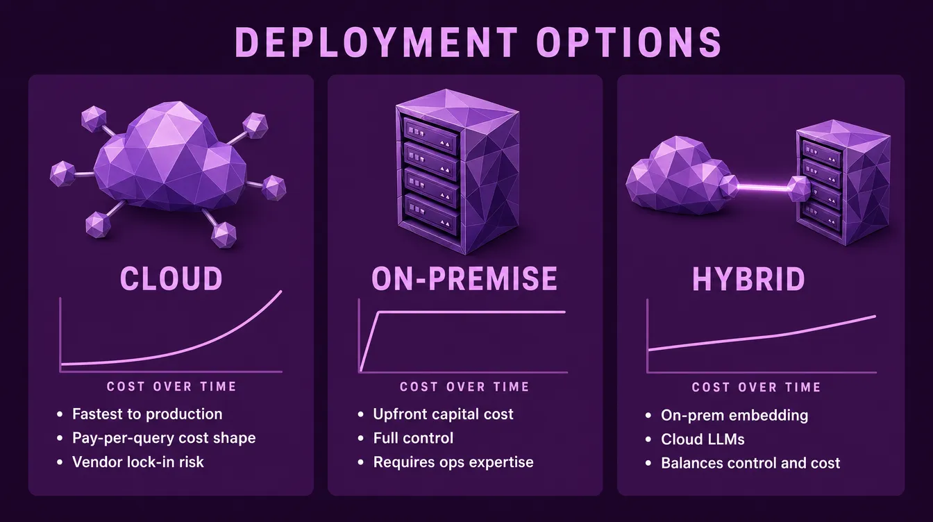
Cost and Infrastructure

RAG infrastructure costs are distributed across components. The deployment model determines the cost shape.

Cloud (managed services): Vector databases (Pinecone, Weaviate, Azure AI Search), embedding APIs (OpenAI, Cohere, Google), and model APIs are the fastest path to production. Costs scale with usage: easy to start, potentially expensive at scale. Managed services handle scaling, availability, and updates. The trade-off is reduced control and vendor lock-in.

On-premise (self-hosted): Open-source embedding models, open-source vector stores (Qdrant, Milvus, pgvector, ChromaDB), and self-hosted LLMs offer full control. Costs are upfront hardware plus operations rather than per-query. The trade-off is required infrastructure expertise and slower iteration.

Hybrid: A common production pattern: on-premise embedding and reranking (where data sensitivity matters), cloud LLMs (where cost-per-query is acceptable). This balances data control with operational cost.

Cost optimization paths, ordered by typical impact:

1. Reduce chunk size (fewer input tokens per query)
2. Optimize retrieval k (fewer chunks sent to the LLM)
3. Choose a smaller generation model (lower per-call inference cost)
4. Batch requests where latency permits (higher throughput per GPU)
5. Cache aggressively (eliminate redundant computation)